Below is something that I posted last year. I posted it for two reasons:

1. I wanted to help others in the same situation.
2. I knew that if I only do this once a year, I forget.

So I read through it again and the letter to the students about missing textbooks and library books is being generated. I hope my crazy steps help make mailing notices to your students easier.

That sounds like one of the most uninteresting titles for an article ever, but it is extremely helpful. At first, my Excel knowledge was something like this (oh, trust me. You need to click on that link). I could impress people for a time as long as things stayed very basic. Then, because of this project, my knowledge of Excel went crazy, something akin to this.

The Problem
Here’s the scenario: one of our school secretaries has a list of students and a list of materials students did not return at the end of the year. Some of these are textbooks and those can reach upwards of $75 in cost. Multiply that by a couple of students and that’s a hefty hit to the budget that the school takes. To counteract that, we send a letter home to families with an invoice of the stuff that needs to be returned to the school.

Some students owe multiple items. In Excel, this showed up as the student’s name being duplicated on as many rows as were items. If a student had three textbooks, that student had three lines of data.

The problem arose when the secretary went to do a mail merge in Word. Each line in Excel generated a new form letter. The wasteful person would be okay printing multiple letters for one student and cramming them in one envelope. We felt like that would be hypocritical, considering we do a paper drive at the beginning of the year and budgets are tight. What do we do?

Enter the Macro
Macros are mini-programs that are perfect for any process that you repeat over and over again. Our secretary was willing to copy and paste from a multi-page PDF into a Word doc for every student. That shows her determination and commitment, but she is super busy as it is and didn’t need a time-waster.

We used two macros and one formula with an end result of one spreadsheet that had the student’s name in column A and his or her owed materials in column B. All of the materials were in one cell and the student only used one line in Excel. The mail merge letter looked beautiful – as beautiful as a mail merge letter can look. To someone freed from a huge copy and paste job, it can be a very beautiful thing.

I decided to combine the textbook list with my library list. If we were mailing students, we might as well only mail one letter. The textbook list had column A formatted First Name Last Name. My library list had Last Name, First Name. Combining lines would be pointless if Test Student was also mentioned as Student, Test in Excel.

Macros can be found in the Developer section of Excel. Most people do not start with the Developer section showing. As with many things in this project, I was unfamiliar with all of the hidden features in Excel. I thought I was slick because I could data sort. Yep. Chimpanzee riding on a Segway.

To enable the Developer section:

Excel 2010
Click on File->Options->Customize Ribbon. Select ‘All Tabs’ from the dropdown and Developer should be in the ‘Main Tabs’ chunk. Click ‘Add’ and then ‘OK’.

Excel 2011
Click on ‘Excel’ in the top menu bar then Preferences->Ribbon. Check ‘Developer’ and hit ‘OK’.

Excel 2008
You are out of luck. Excel 2008 has a Developer section and even looks like it can run macros, just not Visual Basic macros, which is what we’re using for this fix. Our school has Excel 2008, so I had to work at home. You can tell how frustrated people were since Microsoft went back to allowing VBA to execute.

What is VBA?
VBA is Visual Basic for Applications. Gilberto Urroz from Utah State University gives a good explanation here. VBA uses a strain of the Visual Basic programming language to automate certain tasks in different applications, like the Office suite.

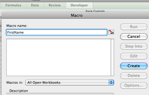
Once you enable the Developer section in Excel, click on that ribbon and then click on ‘Macros’. The first one we’re going to enter is called FirstName (all one word). After you type in the name, click on ‘Create’.

Changing the Formatting to First Name Last Name from Last Name, First Name

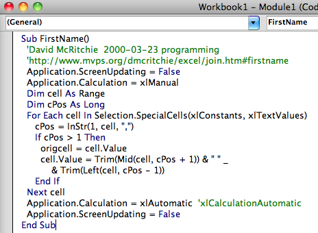
In the macro editor, we are going to paste the following code that I got from David McRitchie:

Sub FirstName()
'David McRitchie 2000-03-23 programming
'http://www.mvps.org/dmcritchie/excel/join.htm#firstname
Application.ScreenUpdating = False
Application.Calculation = xlManual
Dim cell As Range
Dim cPos As Long
For Each cell In Selection.SpecialCells(xlConstants, xlTextValues)
cPos = InStr(1, cell, ",")
If cPos > 1 Then
origcell = cell.Value
cell.Value = Trim(Mid(cell, cPos + 1)) & " " _
& Trim(Left(cell, cPos - 1))
End If
Next cell
Application.Calculation = xlAutomatic 'xlCalculationAutomatic
Application.ScreenUpdating = False
End Sub

It should look like this:

Click on the Play button or click ‘Run’ and it will execute a script that searches column A for commas, flips whatever’s on either side of the comma, and removes the comma.

Now we have all of our names formatted the same way. Next step: combine the book title with the book number and book cost.

Combining multiple cells in one row while keeping the data of each
This step got added when I saw in the mail merge that a couple of teachers had assigned multiple textbooks to a student. When we ran the letter, it said “Test Student has not returned Science 8 and Science 8.” If my student went to our school, I would wonder what crazy things we were teaching her.

The textbook list had column B for the title, column C for the book number (number 13 in a class set of 30 or whatever), and column D for the price. I wanted to combine those.

I used a formula function called ‘concatenate’. A mistake I made was creating the formula inside column B. That deleted the book title checked out to that student. Edit->Undo. In a new column – E for mine – title it “Book + # + Cost”. Title it something that will help you tell the difference between this column and the others.

In E2, I typed:
=CONCATENATE(B:B, " #", C:C, " $", D:D)
and felt pretty awesome, in all honesty.
Concatenating is a fancy way of combining and a lot quicker to type than:
=PUT THAT JUNK TOGETHER NOW OR I WILL PUNCH YOU
which was my next option.

Everything inside the () is a variable for the concatenate function. B:B selects everything in column B, C:C selects C, and D:D selects D. If it said B2, it would only select column B, row 2.

Each variable is separated by a comma. Notice the ” “, between the column variables. I wanted a space between each value when the columns were concatenated, or else it would read “Science 81375″. That would be really confusing, considering it’s Science 8, book 13, and the textbook costs $75.

Anything inside the ” ” Excel will enter as text into the cell. The ” #” puts a number sign in front of column C’s value, which is the book number, and ” $” puts the dollar sign in front of the insane cost publishers charge for textbooks.

E2 now had that formula, but what about the others? You could either copy and paste that formula multiple times or select E2 all the way down to the last row you need (the row for the last student name) and then choose Edit->Fill->Down.

I opened up a new workbook to enjoy this lovely column. I wanted column A to be the student name and a new column B to have the combined book title, number, and cost. I pasted column A from my old sheet to the new without any problem. An error I made was trying to paste column E into the new worksheet’s column B. I tried a regular old paste, so the entire column was full of:
!#REF - I AM DISAPPOINTED IN YOU

Excel can be so condescending at times. Edit->Undo

I then did a Paste Special and chose the Values option. That gave me the final data without having to refer back to any other cells.

I was finally ready to call in the secret weapon.

Merging multiple lines into one line per student
This is where it all started. It’s like a Joseph Campbell monomyth. My quest was initially to get lines to merge, yet the journey to Mount Doom in Mordor was filled with distractors and new challenges. Heavy-hearted, I prepared to cast the One Ring into the flames.

My friend Peter is a computer savant. He’s a great friend and one of the many cool things about him is that he works for Microsoft. He made Office. Hit F1 in Word 2010 and that’s him.

Yes. Peter killed Clippy.

When he found out I needed help, he wrote this elegant piece of code:

Option Explicit

Sub Books()

Dim lastRow, currRowOut, currName, lastBook
lastRow = FindLastRow(ActiveWorkbook.ActiveSheet) + 1
currName = “”
currRowOut = lastRow + 3
lastBook = “”

Dim sheet As Worksheet

Set sheet = ActiveWorkbook.ActiveSheet

Dim r As Integer

For r = 2 To lastRow
If sheet.Cells(r, 1).Value <> currName Then
If sheet.Cells(currRowOut, 2).Value <> “” Then
sheet.Cells(currRowOut, 2).Value = sheet.Cells(currRowOut, 2).Value & “, and ” & lastBook
Else
sheet.Cells(currRowOut, 2).Value = lastBook
End If

currRowOut = currRowOut + 1
currName = sheet.Cells(r, 1).Value
sheet.Cells(currRowOut, 1).Value = currName
lastBook = sheet.Cells(r, 2).Value
Else
If sheet.Cells(currRowOut, 2).Value <> “” Then
sheet.Cells(currRowOut, 2).Value = sheet.Cells(currRowOut, 2).Value & “, ” & lastBook
Else
sheet.Cells(currRowOut, 2).Value = lastBook
End If

lastBook = sheet.Cells(r, 2).Value
End If

Next

End Sub

‘ Finds the last row of actual data in the worksheet… very, very handy.
Function FindLastRow(sheet As Worksheet)
If WorksheetFunction.CountA(sheet.Cells) > 0 Then
‘Search for any entry, by searching backwards by Rows.
FindLastRow = sheet.Cells.Find(What:=”*”, After:=[A1], SearchOrder:=xlByRows, SearchDirection:=xlPrevious).Row
End If
End Function

Create a new macro and name it Books. Paste that bunch of awesomeness into the editor and run it. As long as your worksheet is column A Name, column B Book, you should be good.

The macro will create a new listing four rows down with the single line per student and column B full of each book they owe.

Hopefully this helps us track down those books so students don’t run into trouble at the high school. Sure, it makes the letter easier to understand, but it’s what the families do with that letter that is the bigger importance.

I know that this is a mega-huge post, so feel free to leave comments, questions, and/or links to videos of chimpanzees riding on Segways.

• Previous Entry: A day with Pelican House Productions
• Next Entry: Ray Bradbury – 1920-2012